CRE for Redevelopment Risk: An Earth Observation Exposure Layer In progress
The redevelopment exposure layer is an independent proposal and is not an official U.S. Census Bureau product or project. The Rhode Island proof of concept was developed in part during my Census xD fellowship and used only public data.
An Earth observation exposure layer for the Community Resilience Estimates
-
Joey Marshall — U.S. Census Bureau, SEHSD
SoftwareMethodology
Built the R pipelines for ACS data intake and dasymetric downscaling.
-
Katie Johnson
ConceptualizationSoftwareFormal analysisWriting – original draft
Adapted the pipelines to process multiple ACS vintages; designed and built the geo-temporal model; designed the redevelopment exposure layer.
The Rhode Island proof of concept was developed in collaboration with Joey Marshall and Adel Daoud from the AI & Global Development Lab.
Next-phase design, building on the geo-temporal wealth estimation pipeline (Rhode Island proof of concept)
Problem
A central hypothesis of this project is that satellite imagery can show evidence of displacement before survey data catches up.
Hypotheses this project tests:
- Satellite imagery can reveal redevelopment activity roughly eighteen months before it would show up in survey-based estimates.
- Displacement typically follows visible redevelopment — a sale, a permit, construction — by twelve to thirty-six months.
- Preservation dollars go further the earlier they’re deployed: the same dollar should preserve several times as many units ahead of a repricing as after.
If these hold, a redevelopment exposure layer built from imagery could give housing agencies and tenant advocates meaningfully earlier warning than they have today. None of the three has been validated against ground-truth displacement data yet — they’re the assumptions this project is designed to test, not established findings.
A building sells, permits get pulled, older units come down, larger new ones go up — and, if the displacement-lag hypothesis above holds, rents rise and households leave somewhere between twelve and thirty-six months later. That change doesn’t show up in the ACS, which runs a five-year moving average and is released with a lag, until well after people have already moved and the neighborhood has already changed.
The tools available to people working in real time don’t let them track this as it happens.
State and city housing agencies have to decide how to allocate limited preservation dollars, and it’s a race: affordable housing can be bought and stabilized before prices rise, or bought later at a much higher cost after tenants have already left. Right now those decisions run on permit data where it exists, broker relationships, and judgment.
Community land trusts and CDCs face the same problem with smaller budgets and tighter margins — one bad acquisition can consume a year’s entire budget.
Public housing authorities need to know when voucher holders are losing their housing at the moment it happens, not afterward, so they can intervene with property owners or arrange relocation.
Legal aid organizations and tenant groups typically wait for notices before acting, but right-to-counsel programs, know-your-rights outreach, and rental assistance work far better delivered before a notice goes out — which means they need to know where notices are headed.
Hazard mitigation planners write Local Hazard Mitigation Plans on five-year cycles and prepare BRIC subapplications against benefit-cost rules, using building inventories from survey data that’s often stale in exactly the neighborhoods changing fastest.
Emergency managers need current building counts for evacuation planning and damage assessment — a serious risk if a neighborhood has added 400 units since the last survey.
The core problem is that permit and assessor data is only as good as the municipality that keeps it, and the places with the weakest records are usually the places least equipped to protect their residents. The neighborhoods most at risk of displacement are also the hardest to monitor.
Solution
A redevelopment layer for the Community Resilience Estimates, built on the CRE for Heat structure: social vulnerability from the ACS shown side by side with an externally measured exposure indicator, rather than folded into a single score.
CRE for Heat defines exposure as temperature — measured from physical data, independent of who lives there. This layer defines exposure as turnover in the built environment: construction, demolition, and land-use conversion, measured from satellite imagery. It passes the same test: it makes no inference about anyone’s income, and describes something happening to a place from outside it, not a condition of the people in it.
How it’s built: the supervised task flips the current approach. Instead of inferring a hidden economic variable from imagery, the model detects a physical event that’s directly visible in imagery, using administrative records of that event as labels.
- Labels come from parcel-level redevelopment records — municipal building and demolition permits, changes in assessor improvement value, new-construction flags, certificates of occupancy, and sale transactions — starting with Rhode Island’s statewide GIS system and Providence’s open data portal.
- The model learns detection where records are good and applies it where records are scarce. That’s the whole value of the approach, and it’s an equity argument, not an accuracy one: the product exists to extend visibility into the jurisdictions with the weakest record-keeping.
- Output is a redevelopment-intensity figure per cell per year — units added, units removed, turnover rate — plus threshold flags in the CRE-for-Heat style:
REDEV_2YR,DEMO_FLAG,CONVERSION_FLAG. - LIHTC and project-based Section 8 contract expirations, which HUD records years in advance, become the highest-priority signal the system can generate: redevelopment pressure on a block where affordability covenants expire in thirty months is predictable today.
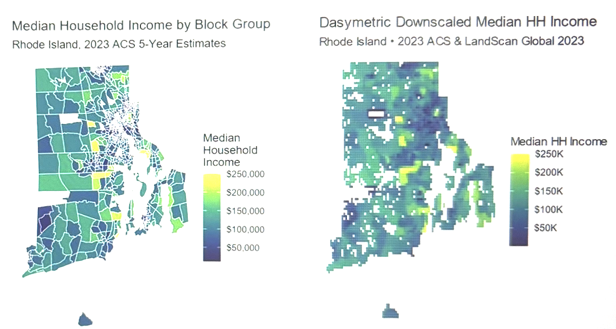
Dasymetric downscaling drops out of the pipeline. This is the biggest simplification. Downscaling existed to solve one problem: the ACS reports at an irregular polygon, the analysis needs a regular grid, so the value gets redistributed across cells using a population proxy. That interpolation step exists only because the reporting geography and the analysis geography don’t match.
The new target removes the mismatch. Permits, demolitions, and assessor records are point events at the parcel level. They sum into a cell rather than needing to be redistributed out of one — the aggregation is exact, where downscaling was always an assumption.
Two sources of error remain: the LandScan weighting still assumes ambient population is a reasonable stand-in for a household-level quantity, and the median-aggregability problem doesn’t go away — counts and valuations aggregate linearly, medians never did.
| Component | Current | New |
|---|---|---|
| Label source | ACS B19013, downscaled | Parcel permits and assessor records, aggregated |
| Geoprocessing | Dasymetric downscaling onto LandScan | Spatial join, parcel → cell |
| Prediction head | Regression on dollars | Count regression or event classification |
| Metrics | R², MAE, RMSE | AUC-PR, precision/recall, count deviance |
| Imagery | Landsat + nightlights, 10 years | Landsat for depth + Sentinel-2 for resolution |
| Key fold | In-country | Out-of-county and out-of-time |
What’s retained: the GEE export infrastructure carries over mostly unchanged. So does the per-cell, per-year TFRecord structure keyed by {i}_{band} — built for exactly this kind of problem. The dual-branch ResNet-18 backbone stays too, and the BiLSTM matters more, not less: redevelopment is a signal that unfolds over time rather than a fixed state, which is why a temporal architecture was the right call from the start.
Two open design questions:
- Resolution. Redevelopment happens at the parcel level. Landsat’s 30-meter resolution can pick up multifamily and commercial builds but misses scattered-site teardowns. Sentinel-2, at 10 meters with a five-day revisit, trades that for a much shorter consistent record — back to roughly 2017, against Landsat’s multi-decade archive. The plan is to use both: Landsat for temporal depth, Sentinel-2 for detection sensitivity in recent years. The 1km cell may also be too coarse; a 250-meter cell is worth testing.
- Class imbalance. Most cell-years show no meaningful redevelopment. The metrics and loss function need to account for that, and R² stops being a meaningful summary statistic here.
Impact
The people above are all active in the window between when redevelopment starts and when displacement happens. That’s the window this changes.
- Preservation acquisitions happen earlier. A housing agency that sees conversion pressure building on a block of naturally occurring affordable housing can buy and secure the properties before the market reprices — the difference between households staying and households having to move. If the preservation-timing hypothesis holds, the same dollar should preserve several times as many units ahead of a repricing as it does after.
- Expiring affordability gets assessed by pressure, not just by date. Every LIHTC covenant eventually expires, but not every expiration is a displacement event. A block with no redevelopment pressure at expiration is a routine administrative process. A block where surrounding properties are being replaced at expiration is an emergency. Right now, both look identical in the HUD database.
- Tenant protection gets staged ahead of the notice. Right-to-counsel programs, door-to-door know-your-rights campaigns, and emergency rental assistance work better before a notice goes out than after. Staging them requires a forecast, and — if the imagery-lead-time hypothesis holds — a physical forecast would be available up to eighteen months before a survey-based one.
- Relocation assistance gets planned instead of improvised. Agencies that know in advance where displacement is coming can prepare for it; agencies that only learn from eviction records can’t.
- Hazard mitigation planning reflects current conditions. A BRIC subapplication built on a stale building inventory omits the fastest-changing neighborhoods — and since BCA requirements penalize undercounted areas, that also makes the application less competitive.
- The visibility gap is smallest where it matters most. A jurisdiction that can’t afford a permit database has no redevelopment data at all today. This model generates that data anyway, from public imagery, at no cost to the jurisdiction — the most direct equity mechanism in the design.
Proof of Concept: What the Current Pipeline Established Proof of concept
The median-income model isn’t just a goal — it’s a complete, reproducible pipeline. The geo-temporal-wealth-estimation-RI system runs the full process end to end: pulls ACS block-group income data and downscales it dasymetrically onto a 1km LandScan grid, exports ten years of Landsat and nightlights composites per cell via Google Earth Engine, builds model-ready TFRecords and cross-validation folds, trains a dual-branch ResNet-18 + BiLSTM model, runs inference on a held-out split, and maps the predictions.
Baseline configuration — frozen ImageNet backbone, in-country fold, evaluated on 1,781 held-out grid cells:
| Metric | Value |
|---|---|
| R² | 0.120 |
| MAE | $24,731 |
| RMSE | $31,300 |
The improvement over a trivial predictor is modest. The test-set label standard deviation is about $33,400 — a model that predicted the statewide average for every cell would land close to that RMSE. This model reaches $31,300: roughly a 6% improvement, about $2,100. The $24,731 MAE is close to a third of Rhode Island’s typical household income. The model has learned something, but not much.
The errors are spread out, not concentrated. The RMSE-to-MAE ratio is 1.27, close to the 1.25 expected under normally distributed errors — the model is uniformly weak across the test set rather than doing well almost everywhere and failing in a few cells. That’s suggestive, though not conclusive (a frozen backbone could produce the same pattern), of a harder explanation: fine-grained income variation within a wealthy, spatially homogeneous state isn’t well reflected in the built environment at 1km resolution.
Why This Is a Step Toward the CRE Design, Not a Detour
The negative result is cleanly localized — it’s the label that failed, not the pipeline. Everything upstream of the regression head worked and carries over directly:
- Google Earth Engine export at scale — roughly 11,900 cells × 10 years × multiple bands, orchestrated and retried.
- A TFRecord schema keyed by
{i}_{band}, built and validated in training, that matters most for a redevelopment model since change detection is inherently a per-timestep problem. - Three fold constructions — in-country, out-of-county, out-of-time — with per-band normalization computed only on each fold’s training set, so leakage stays controlled.
- A dual-branch ResNet-18 + BiLSTM that trains and converges on real labels.
- Inference and map visualization for predicted, actual, and error surfaces.
Most of the engineering carries over unchanged. What changes is the target, the prediction head, the metrics, and the geoprocessing step — which the new target makes unnecessary.
The proof of concept also justified the pivot. Estimating income asks imagery to infer something it can’t see, competes with a survey that’s already better at measuring it, and raises the same disclosure and misuse concerns that come up across AI-for-socioeconomic-prediction work generally. Detecting redevelopment asks imagery to recognize something that’s actually in the pixels, fills a gap no survey covers, and produces an artifact used by the people trying to keep residents in place. An R² of 0.120 is what turned that comparison from theoretical to concrete.
The open question on the income model stays open — whether the gap reflects under-training or a real ceiling. It’s still worth answering, and answering it is now cheap: the pipeline already exists, and closing it out is a matter of tuning, not building.
Disclosure Avoidance
A community land trust deciding which property to buy can use a map of where capital is heading. So can a speculator, using the exact same map for the exact same decision. This layer is a real advance over a decline map because it doesn’t cause a lender to pull back or an insurer to decline renewal — it answers a private buyer’s question of where to acquire before prices move, directly. Disclosure avoidance here has to be designed in before release, not checked afterward.
Standard Census disclosure review is built around re-identifying individuals in survey microdata. Four of the five risks here sit outside that frame:
- Parcel attribution. In a sparsely developed area at Sentinel-2 resolution, a detection can correspond to a single property, and therefore a single owner or household. Higher resolution buys more of this risk along with more accuracy — a disclosure cost as well as a compute cost.
- Unverified claims about identifiable property. The product’s entire purpose is to generate a signal where permit records are scarce, which means asserting that construction or demolition happened at a location with no administrative record to confirm it. That claim can be wrong, and it’s tied to a specific parcel.
- Group inferential disclosure. A well-calibrated flag never identifies an individual, but it can still expose a community to speculative targeting. No one is disclosed — only the neighborhood is — and current DRB practice has no tool for that.
- Composition with CRE’s own protections. CRE publishes at the tract level with margins of error, disclosure-avoided by Census. Pairing tract-level vulnerability with a 250-meter or 1km exposure layer lets a user infer sub-tract structure that CRE deliberately doesn’t publish. The exposure layer can undo the protection built into the host product.
- Lead-time asymmetry. A public release lands on the same day for the buyer and the tenant, but only one of them can act on it within the week.
Controls under consideration:
- A minimum occupied-unit threshold per published cell — cells below it get suppressed, so no published flag maps to a single household.
- A minimum parcel-count threshold at the aggregation level — flags backed by fewer parcels get published at a coarser geography instead, trading resolution for disclosure risk directly.
- An administrative-corroboration rule applied at fine resolution: activity the model flags without a supporting permit or assessor record gets published only at the coarser, cell-level resolution rather than the parcel level.
- A public threshold with a controlled intensity layer: a binary turnover flag reveals far less than exact unit counts and assessed valuations, so the continuous layer moves to controlled access under a data use agreement.
- Rounding and noise injection on any published continuous values.
- A staggered release: preservation actors get the current layer under a data use agreement, and the public release lags behind on a set delay. That removes the speculative lead-time advantage without undermining the use case the product exists for — it’s a policy choice, not a technical one, and it has to be made explicitly.
- An expanded DRB scope covering group-level inferential disclosure, plus a composition check confirming the paired layer doesn’t enable sub-tract inference that CRE withholds.
None of this removes dual use. A layer good enough to help a CDC acquire ahead of a repricing is good enough to help anyone else do the same, and the controls above manage that asymmetry rather than eliminate it. The honest position: the harm profile is better than a decline map, it isn’t clean, and the access-ordering decision is doing most of the protective work.
Stack & Methods
Python (TensorFlow, pandas, numpy, ee) · Google Earth Engine (Landsat, Sentinel-2, VIIRS nightlights) · dual-branch ResNet-18 + bidirectional LSTM (backbone adapted from Pettersson et al., IJCAI 2023) · parcel-level permit and assessor records (RIGIS, municipal open data) · HUD LIHTC and project-based Section 8 contract databases · Census Community Resilience Estimates · out-of-county and out-of-time cross-validation · AUC-PR and count deviance · xD / Data & Society disclosure pre-mortem · Rhode Island proof of concept
AI assistance: Claude (Anthropic) for drafting/editing this description and for code.
Project repository available on GitHub.
Ethics, Data & Limitations
Ethics
See Disclosure Avoidance above for the full privacy-risk and reuse analysis — not duplicated here.
Data Availability
The proof of concept used only public data (ACS, Landsat, VIIRS nightlights, LandScan, Rhode Island GIS). Code is available on GitHub.